Introductory Theory Overview

This section provides a simple crash course on the theory behind market-implied probabilities.

1. Options contain information about future prices

An option is a financial derivative that gives the holder the right, but not the obligation, to buy or sell an asset at a specified price (strike price) on a certain date in the future. Intuitively, the value of an option depends on the probability that it will be profitable or “in-the-money” at expiration. If the probability of ending “in-the-money” (ITM) is high, the option is more valuable. If the probability is low, the option is worth less.

As an example, imagine Apple stock (AAPL) is currently $150, and you buy a call option with a strike price of $160 (meaning you can buy Apple at $160 at expiration).

• If Apple is likely to rise to $170, the option has a high probability of being ITM → more valuable
• If Apple is unlikely to go above $160, the option has little chance of being ITM → less valuable

This illustrates how option prices contain information about the probabilities of the future price of the stock (as determined by market expectations). By knowing the prices of options, we can reverse-engineer and extract information contained about probabilities.

For a simplified worked example, see this excellent blog post. For a complete reading of the financial theory, see this paper.

2. Modelling the volatility surface is crucial to determining probabilities

Using the Breeden-Litzenberger method, the risk-neutral probability density is computed from the second derivative of call prices with respect to strike. In practice, we estimate this derivative numerically from market data. Numerical second derivatives are very sensitive to noise, so noise in observed call price quotes can create large distortions in the implied density.

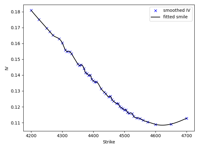Image 1: Directly interpolating observed market prices of call options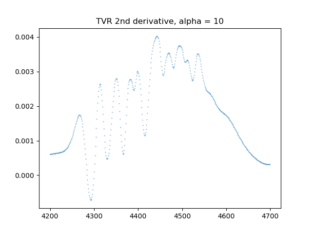

Image 2: Numerical 2nd derivative on noisy market data

Market quotes are noisy and come in discrete increments, which make them unsuitable for numerical differentiation. Instead, we must build a continuous model of theoretical call prices at any strike price, fitted to observed data. We model implied volatility instead of option prices directly because IV is the key input to the pricing model, while prices are a noisier output.

2.1. Implied Volatility (IV)

Implied volatility is the market’s expectation of future price movements of a security. It is the volatility value that, when plugged into an options pricing model (like Black-Scholes), yields the option’s current market price. High IV suggests the market expects significant price swings, while low IV implies a period of relative calm.

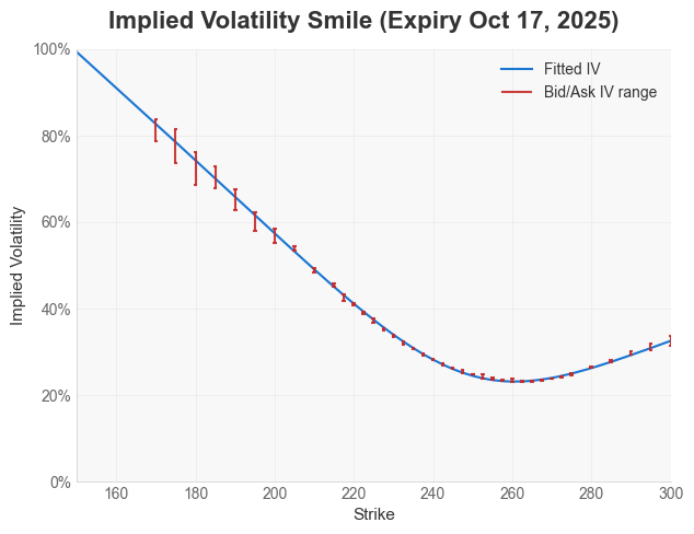
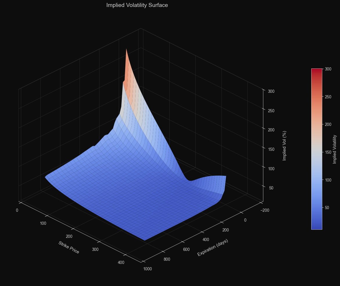
2.2. The Volatility Smile & Surface

• Smile: IV is lowest for at-the-money (ATM) options and increases for both in-the-money (ITM) and out-of-the-money (OTM) options. By plotting IVs against strikes, a “smile” pattern is often observed.

• Surface: We can fit the IV smile repeatedly over many expiries, and interpolate between them to get an IV surface (strike on one axis, time-to-expiry on the other, IV on the vertical axis). While market quotes are only available at discrete points, we can use this fitted surface to estimate IV between quoted strikes and maturities.

A popular academic model used to fit an IV smile is the SVI (Stochastic Volatility Inspired) model. This is the model OIPD relies on. Once we fit the IV surface, we can plug the theoretical IV back into an option pricing model (like Black-Scholes) to determine the price of a call option. Finally, we have a smooth and continuous model of call prices, and this allows us to cleanly take the numerical second derivative.